The meshless finite element method

(*) International Center for Computational Mechanics in Engineering (CIMEC),
Universidad Nacional del Litoral and CONICET, Santa Fe, Argentina

(+) International Center for Numerical Methods in Engineering (CIMNE),
Universitat Politènica de Catalunya, Barcelona, Spain

SUMMARY

A meshless method is presented which has the advantages of the good meshless methods concerning the ease of introduction of node connectivity in a bounded time of order n, and the condition that the shape functions depend only on the node positions. Furthermore, the method proposed also shares several of the advantages of the Finite Element Method such as: (a) the simplicity of the shape functions in a large part of the domain; (b) C⁰ continuity between elements, which allows the treatment of material discontinuities, and (c) ease introduction of the boundary conditions.

KEY WORDS: meshless methods, finite element method, non-Sibsonian interpolation, Delaunay tessellation, natural neighbor co-ordinates

1. INTRODUCTION

The idea of meshless methods for numerical analysis of partial differential equations has become quite popular over the last decade. It is widely acknowledged that 3-D mesh generation remains one of the most man-hours consuming techniques within computational mechanics. The development of a technique that does not require the generation of a mesh for complicated three-dimensional domains is still very appealing. The problem of mesh generation is in fact an automatization issue. The generation time remains unbounded, even using the most sophisticated mesh-generator. Therefore, for a given distribution of points, it is possible to obtain a mesh very quickly, but it may also require several iterations, including manual interaction, to achieve an acceptable mesh.

On the other hand, standard meshless methods need node connectivity to define the interpolations. The accuracy of a meshless method depends, to a great extent, on the node connectivity. Unfortunately, the correct choice of the node connectivity may also be an unbounded problem; in that case, the use of a meshless method may be superfluous.

The definition of the meshless method itself is rather complex. An acceptable definition of meshless methods that takes into account both previous remarks may be: 

A meshless method is an algorithm that satisfies both of the following statements:

I)the definition of the shape functions depends only on the node positions.

II)the evaluation of the nodes connectivity is bounded in time and it depends exclusively on the total number of nodes in the domain.

The first statement is the actual definition of meshless method: everything is related to the node positions. The second statement, on the other hand, is the rationale or the raison d'etre, for using a meshless method: a meshless method is useless without a bounded evaluation of the nodes connectivity.

With the definition given above, the standard Finite Element Method (FEM) is not, of course, a meshless method. The same point distribution in FEM may have different shape functions (the triangulation is not unique) and the evaluation of nodal connectivity does not necessarily have to be bounded in time to yield accurate results (for instance, the Delaunay tessellation is of order n, but it does not necessarily yield accuracy shape functions). On the basis of above, several so-called meshless methods should be revisited in order to verify if they are truly meshless.

In this paper, a generalization of the FEM will be proposed in order to transform it into a meshless method.

2. MESHLESS BACKGROUNDS

Over the last decade a number of meshless methods have been proposed. They can be subdivided in accordance with the definition of the shape functions and/or in accordance with the minimization method of the approximation. The minimization may be via a strong form as in the Point Collocation approach) or a weak form (as in the Galerkin methods).

One of the first meshless methods proposed is the Smooth Particle Hydrodynamics (SPH)[[1]], which was the basis for a more general method known as the Reproducing Kernel Particle Method (RPKM)[[2]]. Starting from a completely different and original idea, the Moving Least Squares shape function (MLSQ)[[3]] has become very popular in the meshless community. More recently, the equivalence between MLSQ and RPKM has been proven, so that both methods may now be considered to be based on the same shape functions [[4]]. The MLSQ shape function has been successfully used in a weak form (Galerkin) with a background grid for the integration domain by Nayroles et al. [3] and, in a more accurate way, by Belytschko and his co-workers [[5],[6]]. Oñate et al. [[7],[8]] used MLSQ in a strong form (Point Collocation) avoiding the background grid. Liu et al. [[9],[10]] have used the RPKM in a weak form, while Aluru [[11]] used it in a strong form. Other authors use different integration rules or weighting functions [[12],[13]]with the same shape functions,.

A newcomer meshless method is the Natural Element Method (NEM). This method is based on the natural neighbor concept to define the shape functions [[14]]. NEM has been used with a weak form by Sukumar et al. [[15]]. The main advantage of this method over the previously used meshless methods is the use of Voronoï diagrams to define the shape functions, which yields a very stable partition. The added advantage is the capability for nodal data interpolation, which facilitates a mean to impose the essential boundary conditions. 

Finally, all the shape functions, including the FEM shape functions, may be defined as Partition of Unity approximations [[16]]. Several other shape functions may also be developed using this concept.

See Figure 1, for a quick comparison of classical 2-D shape functions.

Figure 1: Classical 2-D shape functions for a regular node distribution.

Some of the critical weaknesses of previous meshless methods are:

1)In some cases it is difficult to introduce the essential boundary conditions.

2)For some methods it is laborious to evaluate the shape function derivatives.

3)Often, too many Gauss points are needed to evaluate the weak form.

4)The shape functions usually have a continuity order higher than C⁰. This decreases the convergence of the approximation and makes it more difficult to introduce discontinuities such as those due to heterogeneous material distributions.

5)Some of the methods do not work for irregular point distributions, or need complicated node connectivity to give accurate results.

6)Some methods need n^? operations to define the node connectivity, with ? >>1 or they need an unbounded number of iterations to overcome weakness # 5.

It is probable that some of the drawbacks just mentioned are the reason why several meshless methods have not been successful in 3-D problems.

3. THE EXTENDED DELAUNAY TESSELLATION

The Finite Element Method (FEM) overcomes all of the critical drawbacks described previously with the exception of weakness # 6. We can ask ourselves if it is possible to transform the FEM in order obtain a method which satisfies both of the meshless statements definition. The answer is yes. 

In order to better understand the procedure, classical definitions will be introduced for 3 entities: Voronoï diagrams, Delaunay tessellations and Voronoï spheres.

Let a set of distinct nodes be: N = {n_1, n₂, n₃,?,n_n} in R³.

a)The Voronoï diagram of the set N is a partition of R³ into regions V_i (closed and convex, or unbounded), where each region V_i is associated with a node n_i, such that any point in V_i is closer to n_i (nearest neighbor) than to any other node n_i. See Figure 2 for a 2-D representation. There is a single Voronoï diagram for each set N.

b)A Voronoï sphere within the set N is any sphere, defined by 4 or more nodes, that contains no other node inside. Such spheres are also known as empty circumspheres.

c)A Delaunay tessellation within the set N is a partition of the convex hull ? of all the nodes into regions ?_i such that ? = U ?_{i ,} where each ?_i is the tetrahedron defined by 4 nodes of the same Voronoï sphere. Delaunay tessellations of a set N are not unique, but each tessellation is the dual of the single Voronoï diagram of the set.

Figure 2: Voronoï diagram, Voronoï circle and Delaunay triangulation
for a 4 nodes distribution in 2D.

The computing time required for evaluation of all these 3 entities is of order n^?, with ? ? 1.333. Using a very simple bin organization, the computation time may be reduced to a simple order n.

As stated above, the Delaunay tessellation of a set of nodes is non-unique, and hence, the shape functions based on it do not satisfy the first meshes statement. For the same node distribution, different triangulations (actually tetrahedrations, as it refers to 3-D) are possible. Therefore, an interpolation based on the Delaunay tessellation is sensitive to geometric perturbations of the position of the nodes. On the other hand, its dual, the Voronoï diagram, is unique. Thus, it makes more sense to define meshless shape functions based on the unique Voronoï diagram than on Delaunay tessellations. In Figure 3 two critical case of Delaunay instabilities are represented. One is the case of 4 nodes on the same circle and the other is the case of a node close to a boundary. In both cases, the Voronoï diagram remains almost unchangeable. 

Furthermore, in 3-D problems the Delaunay tessellation may generate several tetrahedra of zero or almost zero volume, which introduces large inaccuracies into the shape function derivatives. This is the reason why a Delaunay tessellation must be improved iteratively in order to obtain a FE mesh. The time to obtain a mesh via a Delaunay tessellation is then an unbounded operation, thus not satisfying the second statement of the meshless definition.

Figure 3: Instabilities on the Delaunay tessellation.
a) Four nodes on the same circle; b) Node close to a boundary.

In order to overcome both of the drawbacks referred to in the above paragraphs, a generalization of the Delaunay tessellation will be defined. The drawbacks appear in the so-called ?degenerated case?, which is the case where more than 4 nodes (or more than 3 nodes in a 2-D problem) are on the same empty sphere. For instance, in 2-D, when 4 nodes are on the same circumference, 2 different triangulations satisfy the Delaunay criterion. However, the most dangerous case appears only in 3-D. For instance, when 5 nodes are on the same sphere, 5 tetrahedra may be defined satisfying the Delaunay criterion, but some of them may have zero or almost zero volumes, called slivers, as seen in Figure 4.

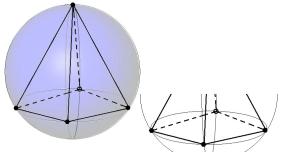
Figure 4: Five nodes on the same sphere and possible zero or almost zero volume tetrahedron (sliver) on the right.

Definition: The Extended Delaunay tessellation within the set N is the unique partition of the convex hull ? of all the nodes into regions ?_i such that ? = U ?_{i ,} whereeach ?_i is the polyhedron defined by all the nodes laying on the same Voronoï sphere.

The main difference between the traditional Delaunay tessellation and the Extended Delaunay tessellation is that, in the latter, all the nodes belonging to the same Voronoï sphere define a unique polyhedron. With this definition, the domain ? will be divided into tetrahedra and other polyhedra, which are unique for a set of node distributions, satisfying then, the first statement of the definition of a meshless method.

Figure 5, for instance, is a 2-D polygon partition with a triangle, a quadrangle and a pentagon. Figure 6 is a classical 8-nodes polyhedron with all the nodes on the same sphere, which may appear in a 3-D problem.

Figure 5: Two-dimensional partition in polygons.
The triangle, the quadrangle and the pentagon are each inscribed on a circle

It must be noted that, for non-uniform node distributions, considering infinite precision, only 4 nodes are necessary to define a sphere. Other nodes close to the sphere may define other spheres very close to the previous one. In order to avoid this situation, which may hide polyhedra with more than 4 nodes, a parameter d will be introduced. In such a way, the polyhedra are defined by all the nodes of the same sphere and nearby spheres with a distance between center points smaller than d. See Appendix I.

Figure 6: Eight-node polyhedron. All nodes are on the same sphere.

The parameter d avoids the possibility of having zero volume or near zero volume tetrahedra. When d is large, the number of polyhedra with more than 4 nodes will increase, and the number of tetrahedra with near zero volume will decrease, and vice versa.

The Extended Delaunay tessellation allows the existence of a domain partition which: (a) is unique for a set of node distributions; (b) is formed by polyhedra with no zero volume, and (c) is obtained in a bounded time of order n. Then, it satisfies the conditions for a meshless method as stated previously.

4. THE SHAPE FUNCTIONS

Once the domain partition in polyhedra is defined, shape functions must be introduced to solve a discrete problem. Limiting the study to second-order elliptic PDE?s such as the Poisson?s equation, C⁰ continuity shape functions are necessary for a weak form solution. If possible, shape functions must be locally supported in order to obtain band matrices. They must also satisfy two criteria in order to have a reasonable convergence order, namely partition of unity and linear completeness. The FEM typically uses linear or quadratic polynomial shape functions, which ensure C⁰ continuity between elements. When the elements are polyhedra with different shapes, polynomial shape functions may only be used for some specific cases. 

In order to define the shape functions inside each polyhedron the non-Sibsonian interpolation will be used [[17]].

Let P = {n₁, n₂, ?, n_m} be the set of nodes belonging to a polyhedron. The shape function N_i(x) corresponding to the node n_i at an internal point x is defined by building first the Voronoï cell corresponding to x in the tessellation of the set P U {x} and then by computing:

(1)

where s_i(x) is the surface of the Voronoï cell face corresponding to node the node n_i and h_i(x) is the distance between point x and the node n_i as seen in Figure 7.

Figure 7: Four nodes and arbitrary internal point x Voronoï diagram. Shape function parameters

Non-Sibsonian interpolations have several properties, which can be found in reference [17]. The main properties are:

1)0 £ N_i(x) £ 1(2)

2)S_i N_i(x) = 1(3)

3)N_i (n_j) = d_ij(4)

4)x = S_i N_i (x) n_i(5)

Furthermore, the particular definition of the non-Sibsonian shape function for the limited set of nodes on the same Voronoï sphere, adds the following properties:

5)On a polyhedron surface, the shape functions depend only on the nodes of this surface [15].

6)On triangular surfaces (or in all the polygon boundaries in 2-D), the shape functions are linear.

7)If the polyhedron is a tetrahedron (or a triangle in 2-D) the shape functions are the linear finite element shape functions.

8)Due to property 5, the shape functions have C⁰ continuity between two neighboring polyhedra. See Figure 8.

9)As a matter of fact, because all the element nodes are on the same sphere, the evaluation of the shape functions and its derivatives becomes very simple (see Appendix II).

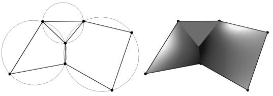
Figure 8: C⁰ continuity of the shape function on a 2-D node connection.

The method defined here is termed the Meshless Finite Element Method (MFEM) because it is both a meshless method and a Finite Element Method. The algorithm steps for the MFEM are:

1)For a set of nodes, compute all the empty spheres with 4 nodes.

2)Generate all the polyhedral elements using the nodes belonging to each sphere and the nodes of all the coincident and nearby spheres (the criterion to choose these spheres is given in Appendix I).

3)Calculate the shape functions and their derivatives, using the non-Sibsonian interpolation, at all the Gauss points necessary to evaluate the integrals of the weak form.

The MFEM is a truly meshless method because the shape functions depend only on the node positions. Furthermore, steps 1 and 2 of the node connectivity process are bounded with n^1.33, avoiding all the mesh "cosmetics" often needed in mesh generators.

Figure 9 shows the shape function and its first derivatives for a node of a 2-D pentagon. The shape function takes the value 1 at a node and 0 at all the other nodes. The linear behavior on the boundaries may be appreciated. 

Figure 9: Shape function and its first derivatives for a typical node of a pentagon 

It is important to remark the important difference between the MFEM shape functions proposed here and the Natural Element Method (NEM) shape functions. Both methods use shape functions based on Voronoï diagrams, but they are completely different. The NEM shape functions have C^? continuity, and are built using the Voronoï diagram of all the natural neighbor nodes to each point xIn this way, very complicated shape functions are obtained which are difficult to differentiate and which need several Gauss points for the numerical computation of the integrals. See Figure 10 for a graphic representation of the NEM and MFEM shape functions.

Figure 10: Shape functions in a 2-D regular node distribution. a) MFEM; b) NEM

The number of Gauss points necessary to compute the element integrals depends, to a great extent, on the polyhedral shape of each element. It must be noted that, for an irregular node distribution, there remains a significant amount of tetrahedra with linear shape functions, for which only one Gauss point is enough. For the remaining polyhedra, the integrals are performed dividing them into tetrahedra and then using a single Gauss point in each tetrahedron. This subdivision is only performed for the evaluation of the integrals.

5. THE BOUNDARY CONDITIONS

Two issues must be taken into account concerning the boundary conditions: the geometric description of the boundary surface and the boundary conditions themselves. 

5.1. Boundary surfaces

One of the main problems in mesh-generation is the correct definition of the domain boundary. Sometimes, boundary surface nodes are explicitly defined as special nodes, which are different from internal nodes. In other cases, the total set of nodes is the only information available and the algorithm must recognize the boundaries. Such is the case for instance, with the Lagrangian formulation of fluid mechanics problems in which, at each time step, a new node distribution is obtained and the free-surface must be recognized from the node positions.

The use of Voronoï diagrams or Voronoï spheres may make it easier to recognize boundary surface nodes. By considering that the node follows a variable h(x) distribution, where h(x) is the minimum distance between two nodes, the following criterion has been used:

All nodes which are on an empty sphere with a radius r(x) bigger than ? h(x), are considered as boundary nodes.

In this criterion, ? is a parameter close to, but greater than one. Note that this criterion is coincident with the Alpha Shape concept [[18],[19]].

Once a decision has been made concerning which of the nodes are on the boundaries, the boundary surface must be defined. It is well known that, in 3-D problems, the surface fitting a number of nodes is not unique. For instance, four boundary nodes on the same sphere may define two different boundary surfaces, one concave and the other convex.

In this paper, the boundary surface is defined with all the polyhedral surfaces having all their nodes on the boundary.

The correct boundary surface may be important to define the correct normal external to the surface. Furthermore; in weak forms it is also important a correct evaluation of the volume domain. Nevertheless, it must be noted that in the criterion proposed above, the error in the boundary surface definition is of order h. This is the standard error of the boundary surface definition in a meshless method for a given node distributions.

5.2. Boundary Conditions

The greatest advantage of the MFEM, which is shared with the FEM, is the easy imposition of the boundary conditions. The essential boundary conditions are introduced directly by imposing a value to the node parameters. The natural zero value condition is imposed automatically without any additional manipulation.

6. NUMERICAL TEST

A cube of unit side, with an internal exponential source, has been used to validate the MFEM.

The problem to be solved is the classical Poisson equation:

Ѳu = f(x, y, z)(6)

With the internal source :

f(x, y, z) =(- 2 k y z (1 - y)(1 - z) + (k y z (1 - y) (1 - z) (1 - 2 x)²)²
- 2 k z x (1 - z)(1 - x) + (k z x (1 - z) (1 - x) (1 - 2 y)²)²
- 2 k x y (1 - x)(1 - y) + (k x y (1 - x) (1 - y) (1 - 2 z)²)² )
(- e^{kxyz (1 - x) (1 - y) (1 - z)} / (1 - e^k/64))(7)

The boundary condition is the unknown function u equal to zero on all the boundaries.

This problem has the following analytical solution:

u(x, y, z) = (1 - e^{kxyz (1 - x) (1 - y) (1 - z)}) / (1 - e^k/64)(8)

Several node distributions have been tested with 125 (5³), 729 (9³), 4,913 (17³), and 35,937 (33³) nodes, with structured and non-structured node distributions.

For the structured node distributions, the following procedure was used to generate the nodes: Initially all the nodes are in a regular position with a constant distance h between neighbor nodes. Then, each internal node has been randomly displaced a distance ? h in order to have an arbitrary, but structured, node distribution. Surface and edge nodes are perturbed but remaining in the surface or the edge, corner nodes were not perturbed.

The 3D non-structured node distribution was generated using the GID pre/post-processing code [[20]] with a constant h distribution. GID generates the nodes using an advancing front technique which guarantees that the minimal distance between two nearby nodes lies between 0.707 h and 1.414 h.

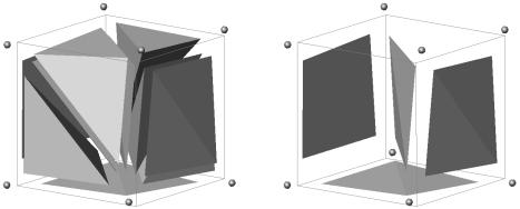
Figure 11: Presence of slivers in a FEM Delaunay partition of a perturbed cube.
Left: Tetrahedra produced by the Delaunay partition. Right: Slivers isolated.

It must be noted that in 2D problems, both node distributions: structured and non-structured, will give a Delaunay partition with near-constant area triangles, which will be optimal for a FEM solution. Nevertheless, this is not the case in 3D problems in which, even for a constant h node distribution, many zero or near-zero volume tetrahedra (slivers) will be obtained on a standard Delaunay partition. Figure 11 shows, for instance, the presence of slivers on a structured eight-node distribution. Slivers may introduce large numerical errors in the solution of the unknowns functions and their derivatives which may completely destroy the solution.

In order to show this behavior and to show that the MFEM eliminates this problem, the following tests were performed: for a fixed-node partition (e.g. 17³ nodes) the dparameter (introduced in section 3 or in equation 11) was swept from 0 to 10^-1. With d= 0 (i.e. Voronoï spheres are never joined) the standard Delaunay tessellation is obtained. Larger values of dgives the extended Delaunay tessellation (Chapter 3) which is the partition used in MFEM.

Figure 12: Cube with exponential source
Error of the derivative in L²-norm, using MFEM for different d.
Left: Structured node distribution with b = 10^-6. Right: Non-structured node distribution.

Figure 12 shows the error in L₂ norm for the derivative of the solution of the 3D problem stated in equations 6 and 7. This has been done both for structured and non-structured distributions against the d parameter. It can be shown that in both cases the errors are very large (~10¹) for d< 10^-6 and very small (~10^-2) for d> 10^-5. Larger d do not change the results.

This example is very important because is showing that, for a given node distribution, a tetrahedrization using the standard Delaunay concept do not work. Mesh generators currently use edge-face swapping or another cosmetic algorithms to overcome the presence of wrong elements. All those operations are unbounded. The idea of joining similar spheres, even for a very small d parameter, solve this problem on a very simple way. The wrong tetrahedra are automatically joined to form polyhedra with optimal shapes in order to be solved by the MFEM.

The results of Figure 12 shows also that d must be large compared with the computer precision (e.g. ~10^-5 for a computer precision of order 10^-16) but also means that d is not a parameter to be adjusted in each example because results does not change by setting d larger than 10^-5. In fact, all our examples were carried out with a fixed d = 10^-1.

From the point of view of the definition of the shape functions, the best polyhedra are those having the following two conditions:

a)All its nodes are on the same empty sphere (this is the concept of optimal distance between nodes).

b)The polyhedra must fill the sphere as much as possible (this is the concept of optimal angle between faces). 

The filling ratio may be defined as:

(9 )

Slivers, for instance, have all their nodes on the same empty sphere, but the g value is near zero. Classical polyhedra as the equilateral tetrahedron has g» 0.12 and for the cube g» 0.37. 

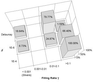
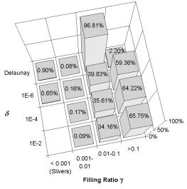
Figure 13: Percentage of polyhedra by volume ratio for different d.
Left: Structured node distribution with b = 10^-6. Right: Non-structured node distribution.

In the Figure 13, for a fixed d, the heights of the columns are representing the percentage of elements having a given filling ratio.

The importance of Figure 13 is to show that, by joining similar spheres, the best polyhedra are automatically built. For instance, small d values lead to some slivers: 18% and 0.90% for d = 0 (Delaunay) and 6.7% and 0.65% for d = 10^-6. Increasing d, the slivers disappears and, in particular for the structured case, all the elements become hexahedra (cubes with g» 0.37), which is the optimal tessellation for this node distribution. For the non-structured case, with d larger than 10^-2, 65% of the elements have a g value greater than 0.10.

Figure 14: Cube with exponential source.
Convergence of the MFEM solution and its gradient for different partitions.
Upper left: Structured node distribution. Upper right: Non-structured node distribution.
Below: Center-line solutions obtained with structured node distribution (the same results were obtained using non-structured node distribution).

Finally, Figure 14 shows the convergence of the MFEM for the example described in equations 6 and 7, when the number of nodes is increased from 5³ to 33³. The upper plots show the error in L²-norm, both for the function and its derivatives. All the graphics shows an excellent convergence rate. It must be noted that for all the non-structured node distributions tested (and also the structured ones for b = 10^-6), the FEM with elements generated using a Delaunay tessellation gave totally wrong results, and several times ill-conditioned matrices were found during the stiffness matrix evaluation.

This example shows the advantages of the MFEM compared with other existing methods in the literature:

a)Compared with the FEM, the advantages are on the mesh generation. In all the examples shown, the node connectivity using the Extended Delaunay Tessellation was generated on a bounded time of order 1.09n, which is the same computer time of the standard Delaunay tetrahedrization. This is a big advantage because the MFEM polyhedra gave excellent results, on the contrary, the standard Delaunay tetrahedra did not worked.

b)Compared with some of the most known meshless methods, the advantage shown by the example is an easy introduction of the essential boundary conditions. The condition u=0 on all the external boundary, was introduced exactly by simply imposing u=0 on all the degrees of freedom of the boundary.

c)One of the main drawbacks of several meshless methods is the evaluation of the integrals of the shape functions and their derivatives. This is not an issue here. For instance, in the non-structured case ~30% of the polyhedra are tetrahedra, which are exactly integrated with only one Gauss point. The remaining polyhedra were divided into tetrahedra made by their faces and its geometric center, and then using one Gauss point at each tetrahedron.

d)Compared with other meshless methods that use point collocation, in which no integration is necessary, the MFEM have all the classical advantages of the Galerkin weighted-residual methods, like symmetric matrices, easy introduction of natural boundary conditions, and more stable and smooth solutions for irregular node distributions.

7. CONCLUSIONS

The Meshless Finite Element Method has been presented. In contrast with other methods found in the literature, the method has the advantages of a good meshless method concerning the ease of introduction of nodes connectivity in a bounded time of order » n, and the condition that the shape functions depends only on the node positions.

Furthermore, the method proposed also shares several of the advantages of the Finite Element Method such as: (a) the simplicity of the shape functions in a large part of the domain; (b) C⁰continuity between elements, which allows the treatment of material discontinuities, (c) an easy introduction of the boundary conditions, and (d) symmetric matrices.

The MFEM can be seen either as a finite element method using elements with different geometric shapes, or as a meshless method with clouds of nodes formed by all the nodes that are in the same empty sphere. In either case, whether as a meshless method or as a standard FEM, the method satisfies the raison d?etre of the meshless procedures: it permits the development of a node connectivity in a bounded time of order n.

Apendix

I. Criterion to join polyhedra

Consider two Voronoï spheres having nearby centers. See Figure 15 for a two dimensional reference.

Figure 15: Four nodes in near-degenerate position showing the empty circumcircles, Voronoï diagram and the corresponding discontinuous Delaunay triangulation.

As both Voronoï spheres are empty, they must satisfy the following relationship:

|r₂ - r₁| £ ||c₁ - c₂||(10)

where r are the radii and c the centers of the spheres.

Thus two spheres are similar when their centers satisfy:

||c₁ - c₂|| < d r_rms,(11)

where d is a small non-dimensional value and r_rms is the root-mean-square radius. Actually comparison are made between two families of similar spheres.

Two polyhedra will be joined if they belong to similar spheres.

The algorithm finds all the 4-node empty spheres, and then polyhedra are successively joined using the above criterion. It must be noted that when all the nodes of a polyhedron belongs to another polyhedron, only the last one is considered.

II. Non-Sibsonian shape functions

For any point within a polyhedron P, there is a Voronoï cell V(x) associated to the variable point x in the Voronoï tessellation of the set PU {x}.

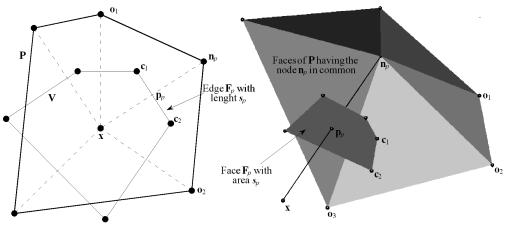
Figure 16: Elements defining 2D and 3D shape functions.

Figure 16 shows that every node n_pÎ P has a corresponding face F_p of V, which is normal to the segment {x, n_p} by its midpoint. This is because V is the set of points closer than x than any other point.

Defining the functions:

f_p(x) = s_p / ||n_p - x|| = s_p / h_p,(12)

as the quotient of s_p, the Lebesgue measure of F_p (s_p); and h_p, the distance between the point x and the node n_p. The shape functions are:

N_p = f_p / S_qf_q,(13)

automatically satisfying the partition of unity property:

S_p N_p = 1.(14)

II.1. Linear completeness

Using the fact that F_p is perpendicular to the vector (n_p - x) the Gauss theorem applied to V gives:

0 = S_pf_p (n_p - x) = S_pf_p n_p - S_pf_p x,(15)

x = S_p [f_p / S_qf_q] n_p = S_p N_p n_p.(16)

Thus non-Sibsonian shape functions are capable of exactly interpolate the variable point x so they have the local coordinate property. By this and the partition of unity property, they can exactly interpolate any linear function:

f(x) = T · x + t = T · (S_p N_p n_p) + t (S_p N_p) = S_p N_p (T ·n_p + t) = S_p N_p f(n_p),(17)

where T is any constant tensor and f any constant vector. This property is known as linear completeness.

II.2. Calculation and derivatives

From now on, the origin will be located at x, so h_p = ||n_p||.

The face F_p of V is made up by the centers {c_q} of the m spheres defined by x, n_p, and two other points from a subset OÌ P.

Calling:

p_p = n_p / 2,(18)

to the midpoint of {x, n_p} and using the symbol Å to represent sum modulus m in the circular ordered set {c_q}, the area of F is the sum of the areas of the triangles {c_q, c_qÅ1, p_p}:

s_p = S_q s_pq.(19)

By the same subdivision process:

f_p = S_qf_pq = S_q(s_pq / h_p),(20)

Each triangle is a face of a tetrahedron {x, p_p, c_q, c_qÅ1} with volume v_pq. By virtue of the perpendicularity between the segment {x, p_p} and the triangle {p_p, c_q, c_qÅ1}:

s_pq = 3 v_pq / (h_p / 2) = (c_q, c_qÅ1, p_p) / h_p = (c_q, c_qÅ1, n_p) / (2 h_p)(21)

with (·, ·, ·) indicating triple product of the vectors enclosed.

Omitting the irrelevant factor 2, the formula:

f_pq = (c_q, c_qÅ1, n_p) / n_p²(22)

is the actual formula used for the computation.

Calling e_i to the Cartesian basis-vectors, ?_jkl to the permutation symbol and ?_i^j to the Kroneker symbol, the derivatives of the shape functions are:

?_i(c_q, c_qÅ1, n_p) = ?_jkl (?_ic^j_q c^k_qÅ1 n^l_p + c^j_q ?_ic^k_qÅ1 n^l_p - c^j_q c^k_qÅ1 ?_i^l)
= (?_ic_qx c_qÅ1 + c_qx ?_ic_qÅ1) · n_p - (c_q, c_qÅ1, e_i)(23)

The derivatives of the centers of a sphere with respect to one of its defining points (?_ic) can be seen in the Apendix III below.

?_in_p² = -2 n_p^j ?_i^j = -2 n_pⁱ(24)

?_if_pq = [(?_ic_qx c_qÅ1 + c_qx ?_ic_qÅ1) · n_p - (c_q, c_qÅ1, e_i)] / n_p² + 2 (c_q, c_qÅ1, n_p) n_pⁱ / n_p⁴(25)

?_if_p = S_q?_if_pq(26)

?_iN_p = (S_q?_if_pqS_rS_sf_rs - S_qf_pqS_rS_s?_if'_rs) / (S_rS_sf_rs)²(27)

III. Derivatives of the sphere center with respect to one of its defining points.

III.1. Circunference

The circumcenter of {x, n^*₀, n^*₁} is:

c = (n₀^{^}n₁² - n₁^{^}n₀²) / 2(n₀x n₁),(28)

where vectors n are n^*- x, and ^{^} means the vector must be counterclockwise rotated 90º:

n_p^{^}j= ?_ij n_pⁱ(29)

Deriving:

?_in_p^j = -?_i^j(30)

?_in_p² = -2 n_p^j ?_i^j = -2 n_pⁱ(31)

?_in_p^{^}j = - ?_kj ?_i^k = - ?_ij(32)

?_i(n₀^{^}j n₁² - n₁^{^}j n₀²) = 2 (n₁^{^}j n₀ⁱ - n₀^{^}j n₁ⁱ) + ?_ij (n₀² - n₁²) (33)

?_i(n₀x n₁) = ?_jk (-?_i^j n₁^k - n₀^j ?_i^k) = ?_ij (n₀ - n₁)^j = (n₁ - n₀)^{^}i(34)

?_ic^j = {[2 (n₁^{^}j n₀ⁱ - n₀^{^}j n₁ⁱ) + ?_ij (n₀² - n₁²)] 2 (n₀x n₁) -
(n₀^{^}j n₁² - n₁^{^}j n₀²) 2 (n₁ - n₀)^{^}k} / 4 (n₀x n₁)² =
= [n₁^{^}j n₀ⁱ - n₀^{^}j n₁ⁱ + ?_ij (n₀² - n₁²) / 2 + c^j (n₀ - n₁)^{^}i ] / (n₀x n₁)(35)

III.2. Sphere

The circumcenter of {x, n^*₀, n^*₁, n^*₂} is:

c = (S_p n_p² n_pÅ1x n_pÅ2) / 2(n₀, n₁, n₂).(36)

where vectors n are n^*- x, and Å means sum modulus three.

Deriving:

                                        ?_in_p^j = -?_i^j(37)

?_in_p² = -2 n_p^j ?_i^j = -2 n_pⁱ(38)

v_p = n_pÅ1x n_pÅ2(39)

?_i v_p^j = ?_pi^j = ?_jkl (-?_i^k n_pÅ2^l - n_pÅ1^k ?_i^l) = [(n_pÅ2 - n_pÅ1) x e_i]^j(40)

?_iS_p n_p² v_p^j = [S_p (n_p² ?_pi^j - 2 n_pⁱ v_p^j)](41)

?_i(n₀, n₁, n₂) = - ?_jkl (?_i^j n^k₁ n^l₂ + n^j₀ ?_i^k n^l₂ + n^j₀ n^k₁ ?_i^l) = - S_p (n_pÅ1x n_pÅ2)ⁱ = -S_p v_pⁱ(42)

?_ic^j = {[S_p (n_p² ?_pi^j - 2 n_pⁱ v_p^j)] (n₀, n₁, n₂) + (S_p n_p² v_p^j) (S_q v_qⁱ)} / 2(n₀, n₁, n₂)²(43)

?_ic= [S_p (n_p² ?_pi / 2 - n_pⁱ v_p) + c (S_q v_qⁱ)] / (n₀, n₁, n₂)(44)

References